Excel formulas for financial modelling with free Excel tools

Excel is a powerful software for financial modeling, Accounting , bookkeeping , etcetera and learning its formulas is crucial for financial analysts. In this blog, we’ll explore the top Excel formulas used in financial modeling. We’ll break down each formula, explain how it works, and show you how to use it effectively and make you know what are excel formulas for financial modelling are used . By the end of this blog, you’ll be able to understand formulas used in financial models and create your own model .

To learn MS- Excel You need to have latest version of Microsoft 365 for practicing new finance functions in excel . Most of the students don’t have latest versions . But don’t worry you can practice excel formulas in microsoft 365 for free in web .

Excel formulas for financial modeling are :

1. NPV (Net Present Value):-

Net Present Value formula helps to calculate the present value of future cash flows. It is a basic formula in financial modelling, as it allows you to decide whether an investment is worth or not , based on the future cash flows it is expected to generate.

NPV formula : =NPV(rate, value1, [value2], …)

Where,

• Rate – Discount Rate at which future cash flows are discounted to their  present value.
•  Value 1 and value 2 – cash flows that are expected to generate in future.

2. IRR (Internal Rate of Return) :- 

Internal Rate of Return helps you to decide how much return you get from an investment. It is also one of the important formulas in financial modelling , because it allows you to compare two or more investment opportunities and decide which is a good investment.  

IRR formula: =IRR(A1:A4)

Where, A1,A4 are cells in which you entered values in excel . A1 is the first year return and A4 is the last year return . Excel will take values from A1 To A4 and calculates cash flows and provides IRR in percentage .

Note :

• Make sure your cash flows are in the correct order and include all periods.
• IRR assumes that the returns are reinvested at the IRR rate.

3. XNPV and XIRR: 

XNPV stands for “Extended Net Present Value ” . It helps you to calculate NPV at regular intervals . It helps to understand value of future cash flows in today’s terms considering the dates of  those cash flows. 

XNPV formula : =XNPV(discount_rate, cash_flows_range, dates_range)

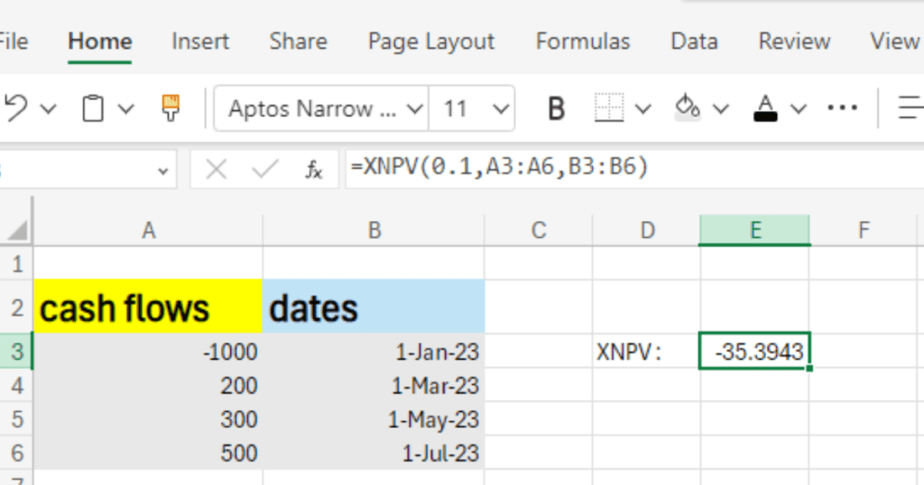
Lets understand XNPV formula with the help of following example : 

1. Click on empty cell where you want the XNPV result to appear.
2. Type the formula: =XNPV(discount_rate, cash_flows_range, dates_range)
3. For example: =XNPV(0.1, A3:A6, B3:B6) (assuming a discount rate of 10%).
4. Press Enter.

XIRR means “Extended Internal Rate of Return” . It helps you to calculate annual rate of return of an investment , Especially when cashflows (money in and money out ) happen in  irregular intervals/ dates . Use XIRR to calculate how much profit you are making during a period but cash flows are not in regular intervals .

XIRR formula : =XIRR(cash_flows_range, dates_range)

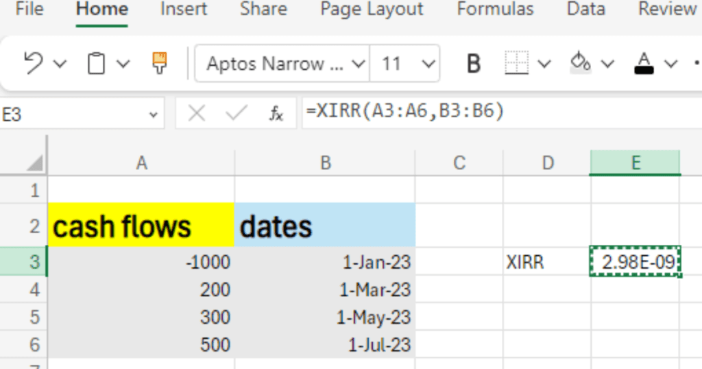
Lets understand XIRR formula with the help of following example : 

1. Click on  empty cell where you want the XIRR result.
2. Type the formula: =XIRR(A3:A6, B3:B6)
3. Press Enter.

4. PMT (Payment): 

PMT stands for “Payment”. PMT formula in excel helps you to calculate payment amount for a loan based on a constant payment or constant interest rates .Use PMT formula when you need to find out the monthly (or any period) payment amount for a loan or investment.

PMT formula : =PMT(rate, nper, pv, [fv], [type])

• Where,
• rate: The interest rate for each period.
• nper: The total number of payment periods.
• pv: The present value or the total amt of the loan.
• fv: (optional) The future value or the balance you want after the last payment (usually 0).
• type: (optional) When payments are due. Use 0 for end of the period (default) and 1 for beginning.

Lets understand PMT formula with the help of following example :

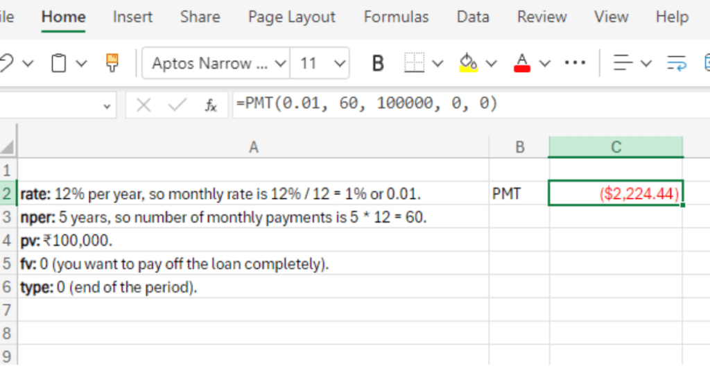
For example you took a loan of ₹100,000 at an annual interest rate of 12%, to be repaid over 5 years with monthly payments.

• rate: 12% per year, so monthly rate is 12% / 12 = 1% or 0.01.
• nper: 5 years, so number of monthly payments is 5 * 12 = 60.
• pv: ₹100,000.
• fv: 0 (you want to pay off the loan completely).
• type: 0 (end of the period).

In Excel, enter: =PMT(0.01, 60, 100000, 0, 0)

Press Enter, and you’ll get the monthly payment amount.

Related PMT formulas : 

IPMT (Interest):

IPMT formula calculates interest for a period.

Formula: =IPMT(rate, per, nper, pv, [fv], [type])

PPMT (Principal):

PPMT formula calculates principal for a period.

Formula: =PPMT(rate, per, nper, pv, [fv], [type])

FV (Future Value):

FV formula calculates future value of an investment for a given period, constant payments and constant interest rate.

Formula: =FV(rate, nper, pmt, [pv], [type]

5. VLOOKUP AND XLOOKUP :

Lookup functions in excel are very important because it is used in various parts in financial models and other fundamental analysis. The LOOKUP function helps you to find a value from a column or in a row . lookup has been powered with vertical , horizontal and x searches . important lookup formulas are : 

VLOOKUP stands for “Vertical Lookup.” It is a function in Excel used to find a value in the first column of a table and return a value in the same row from a specified column.

VLOOKUP formula: =VLOOKUP(lookup_value, table_array, col_index_num, [range_lookup])

Where,

• lookup_value: The value you want to search .
• table_array: The range of cells that contains the data (e.g., A1).
• col_index_num: The column number in the table from which you want to retrieve the value.
• [range_lookup]: Optional. TRUE for an approximate match or FALSE for an exact match.

Lets understand VLOOKUP formula with the help of following example : 

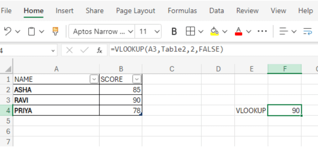
To find Ravi’s score, you use: =VLOOKUP(“Ravi”, A2:B4, 2, FALSE)

• “Ravi” is the lookup_value.
• A2:B4 is the table_array.
• 2 is the col_index_num because the score is in the second column.
• FALSE means  exact match.

The result will be 90.

XLOOKUP is a more flexible and powerful version of VLOOKUP, available in newer versions of Excel (Excel 360). It can search both vertically and horizontally and offers more options.

Formula: =XLOOKUP(lookup_value, lookup_array, return_array, [if_not_found], [match_mode], [search_mode])

Where,

• lookup_value: The value you are searching for.
• lookup_array: The range of cells to search.
• return_array: The range of cells that contains the value to return.
• [if_not_found]: Optional. The value to return when no match is found.
• [match_mode]: Optional. type of match (exact, approximate, etc.).
• [search_mode]: Optional. Specifies the search mode (first-to-last or last-to-first)

Lets understand XLOOKUP formula with the help of following example :

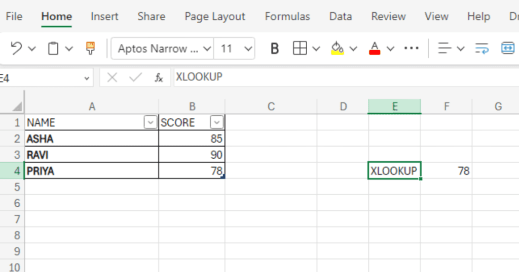
To find Priya’s score, you use: =XLOOKUP(“Priya”, A2:A4, B2:B4, “Not Found”)

• “Priya” is the lookup_value.
• A2:A4 is the lookup_array (names).
• B2:B4 is the return_array (scores).
• “Not Found” is the value returned if there is no match.

The result will be 78.

learn more about MS_excel here…